Developing a D3.js Edge

1. Standard D3

Introduction to an example of a typical D3 chart
Explanation of the key D3 elements used
Illustration of issues arising from re-using a standard chart

If you work through the D3.js tutorials and the D3.js examples, you'll eventually become familiar with a typical way of using D3.js. By this we mean with a set of techniques, and code structures that most people frequently use when working with D3.js. These techniques and code strucutures work great for demonstrating the core concepts of D3.js to those just learning and implementing one-off visualizations. However, as it is their main focus to demonstrate core concepts, they often don't address the problem of creating more than one visualization efficiently. Somebody just learning D3.js would most likely be tempted to simply copy and paste the code used to create a visualization when they need another one that uses new data, perhaps unware that there is a better way. A way that is really the essence of the D3.js. Before we demonstrate this better way, let's first take a look of this "typical" standard D3 use, and some of the pitfalls of re-use following this pattern.

A Typical D3 Chart

Rather than re-invent the wheel, we've taken a typical example of how to use D3.js, and provided a walkthrough of its constituent parts and how they all relate to one another:

Typical D3 Bar Chart

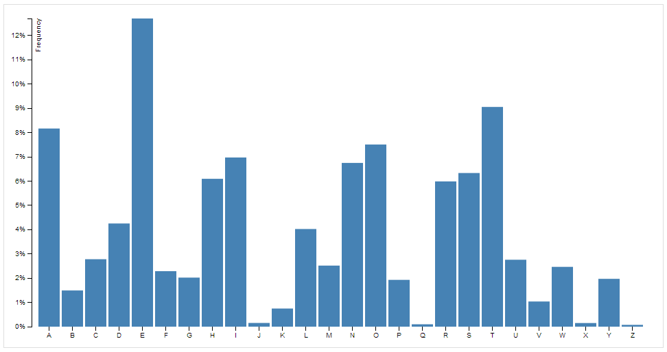
The above is a simple bar chart illustrating the frequency that letters of the alphabet appear in some text.

code/Chapter01/TypicalBarChart/

The data is a simple .tsv (Tab Separated Values) file, with one column for letters and one column for the frequency of occurrence of the letters in the text:

001:letter frequency
002:A .08167
003:B .01492
004:C .02780
005:D .04253
006:E .12702

The source code that generates the above chart is listed in full next (we walk through the entire code right after this source code):

001:var margin = {top: 20, right: 20, bottom: 30, left: 40},
002:        width = 960 - margin.left - margin.right,
003:        height = 500 - margin.top - margin.bottom;
004:
005:    var formatPercent = d3.format(".0%");
006:
007:    var x = d3.scale.ordinal()
008:        .rangeRoundBands([0, width], .1);
009:
010:    var y = d3.scale.linear()
011:        .range([height, 0]);
012:
013:    var xAxis = d3.svg.axis()
014:        .scale(x)
015:        .orient("bottom");
016:
017:    var yAxis = d3.svg.axis()
018:        .scale(y)
019:        .orient("left")
020:        .tickFormat(formatPercent);
021:
022:    var svg = d3.select("#figure").append("svg")
023:        .attr("width", width + margin.left + margin.right)
024:        .attr("height", height + margin.top + margin.bottom)
025:        .append("g")
026:        .attr("transform", "translate(" + margin.left + "," + margin.top + ")");
027:
028:    d3.tsv("data.tsv", function(error, data) {
029:
030:        data.forEach(function(d) {
031:            d.frequency = +d.frequency;
032:        });
033:
034:        x.domain(data.map(function(d) { return d.letter; }));
035:        y.domain([0, d3.max(data, function(d) { return d.frequency; })]);
036:
037:        svg.append("g")
038:            .attr("class", "x axis")
039:            .attr("transform", "translate(0," + height + ")")
040:            .call(xAxis);
041:
042:        svg.append("g")
043:            .attr("class", "y axis")
044:            .call(yAxis)
045:            .append("text")
046:            .attr("transform", "rotate(-90)")
047:            .attr("y", 6)
048:            .attr("dy", ".71em")
049:            .style("text-anchor", "end")
050:            .text("Frequency");
051:
052:        svg.selectAll(".bar")
053:            .data(data)
054:            .enter().append("rect")
055:            .attr("class", "bar")
056:            .attr("x", function(d) { return x(d.letter); })
057:            .attr("width", x.rangeBand())
058:            .attr("y", function(d) { return y(d.frequency); })
059:            .attr("height", function(d) { return height - y(d.frequency); });

The first significant chunk of code sets some chart attributes and builds a scale using a reusable scale function and an axis using one of the most important reusable components of the D3.js core (d3.axis).

Walkthrough of the Code

A margin object (see Mike Bostocks 'conventional margins' approach to margins ) is set up, plus the resulting width and height of the final chart, which uses the values defined in the margin object:

001:var margin = {
002:        top: 20,
003:        right: 20,
004:        bottom: 30,
005:        left: 40
006:    },
007:    width = 960 - margin.left - margin.right,
008:    height = 500 - margin.top - margin.bottom;

The D3.js format function generates a format function, which in turn is used later on to format the percentages as easy-on-the-eye human readable percentages on the y-axis. D3.js often uses this pattern; a configurable function returning a function to be used on the data:
```
001:var formatPercent = d3.format(".0%");
```
The ordinal scale function is used to create an ordinal scale object for the x-axis (i.e. the letters). The code also defines the output range of the ordinal scale object, between zero and width, using the rangeRoundBands attribute.

Note that at this stage the x ordinal scale object has not yet been provided with any input domain, i.e. it doesn't yet know what it is mapping from. This bit only defines what it is mapping to.

The rangeRoundBands attribute tells the scale to divide the range of output values into blocks, or bands, based upon the number of values in in the input domain.
```
001:var x = d3.scale.ordinal()
002:    .rangeRoundBands([0, width], .1);
```
The next bit of code creates a linear scale object to be used for the y-axis (i.e. to visually represent the frequency-of-occurrence percentage associated with each letter). No input domain is defined at this point, since the domain is defined later on in the code.

Note also that the output range of the y scale is from height to zero, not from zero to height. Each bar is drawn as a rectangle, specifying the x,y of the rectangle (top-left of the rectangle), and the width and the height.

The SVG co-ordinate system has x-axis values increasing horizontally from left to right, and y-axis values increasing from top to bottom of the screen; whereas the co-ordinate system of the chart we wish to render has y-axis values increasing vertically up the screen.

So, the scale to be used for the y-axis is inverted, i.e. from height to zero.
```
001:var y = d3.scale.linear()
002:    .range([height, 0]);
```
Next, the code uses the d3.svg.axis components to create an axis object for the x-axis. The scale attribute of the axis object is set to the ordinal scale we created above.

The orient attribute is interesting and worth a little note. Later on in the code a g SVG element is created to render (i.e. display) the actual x-axis. This g element is shifted to the bottom of the chart (height pixels down the page) using a transform call. The orient attribute of the xAxis object states how the xAxis object will be positioned relative to this g element. In this case it's at the bottom of the g element:
```
001:var xAxis = d3.svg.axis()
002:    .scale(x)
003:    .orient("bottom");
```
Next, the code creates a yAxis object for the y-axis, orientates the yAxis object to the left of the g element created for the y-axis, and passes the format function created earlier to format the percentage values on the y-axis:
```
001:var yAxis = d3.svg.axis()
002:    .scale(y)
003:    .orient("left");
004:    .tickFormat(formatPercent);
```

The next bit of code creates the main SVG element in which the bar chart will itself be rendered, specifying its width and height. It appends a g element, and shifts—using the transform and translate functions—the g element down and right using values from the margin object:

001:var svg = d3.select("body").append("svg")
002:    .attr("width", width + margin.left + margin.right)
003:    .attr("height", height + margin.top + margin.bottom)
004:    .append("g")
005:    .attr("transform", "translate(" + margin.left + "," + margin.top + ")");

Now we get to the code that actually starts to use the data.

The d3.tsv component loads up the data from the data.tsv file and calls the anonymous callback function that starts processing the data:
```
001:d3.tsv("data.tsv", function(error, data) {
```
Remember that the x and y variables are the ordinal and linear scale objects, and are used to provide the xAxis and yAxis objects with the data that those axis objects will actually render. Here the code defines the actual input data for those scale objects.

First up the code uses the Array.map method to create an array of just the letters themselves from the data. This array of letters is then used to define the ordinal input domain of the x scale object:
```
001:x.domain(data.map(function(d) { return d.letter; }));
```
Second, the code defines the input values (i.e. the letter frequency values) to be used in the y linear scale object. The y linear scale object then maps from those input values to the pixel range specified earlier when the y linear scale object was declared. Remembering how the y scale object is defined earlier on, y(0) will return a value of 450 (height), and y(0.12702) will return zero (0.12702 being the maximum frequency):
```
001:y.domain([0, d3.max(data, function(d) { return d.frequency; })]);
```
Next up, the code creates a g element in which the visual elements of the x-axis will be rendered. The g object is assigned the CSS class ("x axis"), and is shifted down the page height pixels, and finishes off with a JavaScript call to the xAxis object. This renders the actual visual x-axis within this g element:
```
001:svg.append("g")
002:    .attr("class", "x axis")
003:    .attr("transform", "translate(0," + height + ")")
004:    .call(xAxis);
```
Similar code follows for the actual visual y-axis, except with a little more going on. First up, the g element used to render the y-axis is created, and the yAxis object is called to render the actual visual y-axis within this g element.

Note that the actual g element is not transformed and shifted; however don't forget that when the yAxis was created, the orientation was specified as "left." So, there was actually no need to transform the actual g element.

The code then appends a text element, transforms this text element ninety degrees anti-clockwise, shifts it a few pixels to the right (using the y and dy attributes), aligns the actual text of the text element, and finally specifies the actual text used within the text element. The dy attribute is being used to transform the text so that the rotation point is on the baseline of the typeface, instead of being at the topmost point of the typeface.
```
001:svg.append("g")
002:    .attr("class", "y axis")
003:    .call(yAxis)
004:    .append("text")
005:    .attr("transform", "rotate(-90)")
006:    .attr("y", 6)
007:    .attr("dy", ".71em")
008:    .style("text-anchor", "end")
009:    .text("Frequency");
```
The last chunk of code is the actual creation of the "bars" in the bar chart. It's in this block of code where we come across an example of the enter/update/exit pattern that you will have encountered in D3.js tutorials and examples.

The selectAll attempts to select all SVG elements with the CSS "bar" class - but there aren't any. The .data() method specifies which data the following code will be applied to, which in this case is the contents of the .tsv file. The enter states that for any "bar" elements not yet created (which in this case is all of them), append an SVG rect element.

For each SVG rect element, assign the bar CSS class and assign the x co-ordinate by mapping from letter to pixel using the x-scale. You then specify the width again using the x-scale, assigning the y coordinate and the height using the y-scale.
```
001:svg.selectAll(".bar")
002:    .data(data)
003:    .enter().append("rect")
004:        .attr("class", "bar")
005:        .attr("x", function(d) { return x(d.letter); })
006:        .attr("width", x.rangeBand())
007:        .attr("y", function(d) { return y(d.frequency); })
008:        .attr("height", function(d) { return height - y(d.frequency); });
```

That's it! This is a typical D3 chart.

Creating Multiple Instances of the Chart

Now, how about if you want to use the above code to create more than one bar chart on the same page? Chances are, your first instinct would be to simply copy and paste the code, and modify the data. Take a look at code/Chapter01/TwoBarCharts. This takes a simplified version of the above bar chart and effectively copies and pastes the code to create two charts.

Here is a glimpse at the code to make two charts:

001:var data1 = [10, 20, 30, 40];
002:
003:var w = 400,
004:    h = 300,
005:    margins = {left:50, top:50, right:50, bottom: 50},
006:    x1 = d3.scale.ordinal().rangeBands([0, w]).domain(data1);
007:    y1 = d3.scale.linear().range([h,0]).domain([0, d3.max(data1)]);
008:
009:var chart1 = d3.select("#container1").append("svg")
010:      .attr('class', 'chart1')
011:      .attr('w', w)
012:      .attr('h', h)
013:    .append('g')
014:      .attr('transform', 'translate(' + margins.left + ',' + margins.top + ')');
015:
016:  chart1.selectAll(".bar")
017:      .data(data1)
018:    .enter().append("rect")
019:      .attr('class', 'bar')
020:      .attr('x', function (d, i) {return  x1(d);})
021:      .attr('y', function (d) {return y1(d);})
022:      .attr('height', function (d) {return h-y1(d);})
023:      .attr('width', x1.rangeBand())
024:      .on('mouseover', function (d,i) {
025:        d3.selectAll('text').remove();
026:        chart1.append('text')
027:          .text(d)
028:          .attr('x', function () {return  x1(d) + (x1.rangeBand()/2);})
029:          .attr('y', function () {return y1(d)- 5;})
030:      });
031:
032:var data2 = [100, 259, 332, 435, 905, 429];
033:
034:var w = 400,
035:    h = 300,
036:    margins = {left:50, top:50, right:50, bottom: 50},
037:    x2 = d3.scale.ordinal().rangeBands([0, w]).domain(data2);
038:    y2 = d3.scale.linear().range([h,0]).domain([0, d3.max(data2)]);
039:
040:var chart2 = d3.select("#container2").append("svg")
041:      .attr('class', 'chart2')
042:      .attr('w', w)
043:      .attr('h', h)
044:    .append('g')
045:      .attr('transform', 'translate(' + margins.left + ',' + margins.top + ')');
046:
047:  chart2.selectAll(".bar")
048:      .data(data2)
049:    .enter().append("rect")
050:      .attr('class', 'bar')
051:      .attr('x', function (d, i) {return  x2(d);})
052:      .attr('y', function (d) {return y2(d);})
053:      .attr('height', function (d) {return h-y2(d);})
054:      .attr('width', x2.rangeBand())
055:      .on('mouseover', function (d,i) {
056:        d3.selectAll('text').remove();
057:        chart2.append('text')
058:          .text(d)
059:          .attr('x', function () {return  x2(d) + (x2.rangeBand()/2);})
060:          .attr('y', function () {return y2(d)- 5;})
061:      });

As you can see, there is a lot of repetition that goes into making these two charts. Actually, the only difference in the code for each chart, is the data that is used to generate them. It seems rather inefficient to copy and paste code whenever you want to a new instance of a chart. What would happen if we wanted 10 charts, each using a different data set. That would be a lot of duplicated code!

Reuse Or Not To Reuse

The above two-chart code does work as it should, so you may well wonder what's the problem? If you were just creating this one page, with just these two bar charts, and you were never going to create D3.js bar charts again, then this approach is probably OK.

However, imagine that you then wished to create another bar chart on a different page. And then imagine that you wished to change something, for example the layout, or the data-format changed. You would then suddenly have three separate blobs of code to update: three places where you can make three different sets of mistakes.

So the question is: how to take this standard approach to creating a D3.js chart—which clearly works—and make it more usable, more straightforward to maintain, and more suitable for sharing with a wider audience?

These are questions that we look to answer in the following chapters.

Summary

Clearly the classic approach to using D3.js works, but we've seen how such an approach doesn't lend itself to elegant, straightforward, easily maintainable, and resuable code.